Monitoring and Measuring Plant Communities
Summary of the more technical quantitative biomonitoring strategies done by professional ecologists and botanists.
Quantitative analysis of the impact of any prairie management effort is essential to determine whether one is doing the right things. This is particularly important when one proceeds with prairie reconstruction work, but it also is vital for monitoring good quality remnants. We prefer the simpler FQA methods for routine use, but here we’ll summarize what the pros do.
Note: this discussion is largely draws from the definitive work by Elzinga et al.: Measuring and Monitoring Plant Populations (5.2MB PDF).
Objectives
The first and most important step is to define the operative goals for prairie management. Typical goals that we’ve set include
- Maximize biodiversity
- Maximize biological quality
- Produce seed
- Produce hay
- Develop savanna regions — buffers between forest and prairie
- Increase natural history knowledge
Beyond these management goals, it’s important to define monitoring objectives_ which are really fairly simple (we want to know what we’ve got, how much of it there is, and how things are changing over time) but can involve a number of things:
- Simplicity — a process easy enough to do that we’ll do it as frequently and comprehensively as needed
- Reproducibility — a process that each of us will be able to do nearly the same way from time to time so that we can reliably combine our results. * Automation — a process that allows us to “touch” each data point only once while entering it into an online automated data management system that will handle the bulk of the work
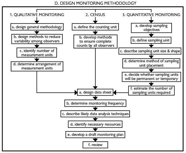
Measurement Design Concepts
Ecologists have defined several constructs to measure how much of something is in a defined area and what it’s “value” is. The important concepts concern sampling strategies, metrics, and biological “value” factors.
Several factors go into any plan for monitoring:
- Frequency of measures — how often do we go out in the field?
- Intensity of measures — how closely do we peer to each spot?
- Interventions and controls — do we compare areas where we do something against areas where we don’t, and how do we match them?
Here is a summary of the methodological approaches for these varying levels of rigor:
Measurement Techniques
Depending on how obsessive we are and how much time we have to do studies, each sample we collect can cover:
- Plots: usually a one hectare = 1/4 acre = 100×100 feet
- Transects: usually a 50 feet linear sample along a tape measure
- Quadrats: usually a 0.25 square meter area — eg a square 0.5 meter on a side or a circle 1.57 meters in diameter
A square quadrat has the advantage of being easy to define with a wooden frame that can be collapsed for easy carrying. Multiple quadrat samples in a plot can be performed along a “strip” within a plot. The distance in from the edge to the first quadrat can be selected randomly, and then subsequent quadrats in the “strip” can be done at regular intervals. This randomizes the inevitable sampling errors from date to date.
The more quadrats that are measured, the more accurate the data. But practically speaking, there needs to be a compromise between the number of quadrats and the degree of detail with which they’re examined. Whether you look briefly at a lot of quadrats or get down on your hands and knees for just a few of them depends on what the question is that you’re trying to answer.
Which leads to the question of what gets measured within each quadrat. There are several alternatives, depending again on the granularity of data needed — which in turn depends on what we’re measuring.
The appropriate measured attribute may be qualitative, semi-quantitative, or quantitative. Selection of the attributes depends on the life history and morphology of what we’re measuring and the resources we can bring to bear. Estimates of what rates of change are significant need to be considered, as well as what we’d do with the information once we’ve got it. (Remember Gertrude Stein’s immortal words: “A difference, to be a difference, must make a difference.”)
Options in more or less increasing rigor include:
- presence or absence of species
- estimates of cover by cover class
- visual esimates of population size
- density of individuals
- cover by percentages
- frequency
- production
Metrics
So here are some metrics in greater detail:
Relative Frequency (RF)
Relative Frequency is the ratio of how many samples a given species is found within divided by the total number of sample-findings of all species. Thus: if we look at three samples and find Species A in one sample and Specie B in all three samples, then we found four total species in all samples, and
- RF of Species A = 1/4 = 0.25 (or 25%)
- RF of Species B = 3/4 = 0.75 (or 75%)
The RF is useful because it is the quickest and easiest determindation; if you see it, you count it whether you see a single individual or a mass of them. But it is a quantitatively crude measure. Consequently, we can also define…
Relative Cover (RC)
Relative Cover is the ratio of “how much” of a given species is summed over all the samples, divided by “how much” of every species is summed over all the samples. This measure requires some quantitation beyond “there or not”. In order of increasing precision, we can report out RC as:
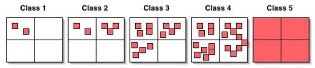
Coverage Classes
- Class 1: species has one to a few stems in only 1 quarter of a quadrat ## Class 2: species has several stems in 1-2 quarters of a quadrat
- Class 3: species has significant presence in 2-3 quarters of a quadrat
- Class 4: species occupies most of 3-4 quarters of a quadrat
- Class 5: species dominates entire quadrat
Coverage Bins
Percentages lumped into “bins” thus:
- Species covers 1-10% of quadrat
- Species covers 11-30% of quadrat
- Species covers 31-50% of quadrat
- Species covers 51-100% of quadrat
Coverage Percentages
Actual percentage, ie a number from 0 to 100. This is an estimate, unless a transet tape is used and literally the number of linear inches covered by each species is recorded. This is the most precise but also by far the most tedious metric.
Relative Importance (RI)
The sum of the RF plus the RC (a number from 0-200) often divided by 2 (to produce a 0-100 scale). The RI combines the rough “present or not” measure with the quantity estimate to improve the accuracy of the estimate. Of course, to calculate a RI when using RC “bin” or “class” measures, you have to convert the bin or class into an actual percentage. This introduces a certain systematic bit of skankiness, but as long as it’s consistently done, this is OK.
So far, these constructs tell us what we’ve got and how much of it there is in relation to everything else there. But these constructs don’t inform us whether this is good or bad. This is of course related to the definition that a weed is a plant whose virtues have not yet been discovered.
However, botanists studying specific locales compile estimates of the “worthiness” of plants found there to create another metric, and that’s where the FQAs come into play.
Created: July 18, 2009 19:01
Last updated: May 26, 2019 17:03
Comments
No comments yet.
To comment, you must log in first.